Tidymodels로 시작하는 머신러닝 (5)

개요

Case Study를 통해 지금까지 익혔던 Tidymodel을 복습합니다.
이 문서는공식영문서를 참조하여 만들었습니다.

관련 포스트
목차

Hotel Booking Data

호텔데이터는 자녀가 있는 가족이 어느 호텔에 머무르는지 예측하기 위한 데이터입니다. Data Dictionary를 참고하면서 데이터의 컬럼과 데이터 타입을 파악하시면 좋습니다.

library를 먼저 불러들입니다.

library(tidymodels)  

# Helper packages
library(readr)       # for importing data
library(vip)         # for variable importance plots

그 다음으로, read_r::read_csv()패키지를 통해서 웹 상에 있는 CSV 데이터를 로드해보겠습니다.

library(tidymodels)
library(readr)

hotels <- 
  read_csv('https://tidymodels.org/start/case-study/hotels.csv') %>%
  mutate_if(is.character, as.factor) 

## 
## -- Column specification ----------------------------------------------------------------------------------
## cols(
##   .default = col_character(),
##   lead_time = col_double(),
##   stays_in_weekend_nights = col_double(),
##   stays_in_week_nights = col_double(),
##   adults = col_double(),
##   is_repeated_guest = col_double(),
##   previous_cancellations = col_double(),
##   previous_bookings_not_canceled = col_double(),
##   booking_changes = col_double(),
##   days_in_waiting_list = col_double(),
##   average_daily_rate = col_double(),
##   total_of_special_requests = col_double(),
##   arrival_date = col_date(format = "")
## )
## i Use `spec()` for the full column specifications.

dim(hotels)

## [1] 50000    23

이 데이터의 주의사항으로 호텔 예약을 취소한 그룹과 취소하지 않은 그룹의 변수(Variables)의 분포가 다르다고 합니다.
지금 로드된 데이터는 호텔 예약을 취소하지 않은 고객에 대해서만 데이터가 수집되어 있습니다.

glimpse(hotels)

## Rows: 50,000
## Columns: 23
## $ hotel                          [3m[38;5;246m<fct>[39m[23m City_Hotel, City_Hotel, Resort_Hotel, Resort_Hotel, Resort_Hotel,~
## $ lead_time                      [3m[38;5;246m<dbl>[39m[23m 217, 2, 95, 143, 136, 67, 47, 56, 80, 6, 130, 27, 16, 46, 297, 42~
## $ stays_in_weekend_nights        [3m[38;5;246m<dbl>[39m[23m 1, 0, 2, 2, 1, 2, 0, 0, 0, 2, 1, 0, 1, 0, 1, 1, 1, 4, 1, 1, 2, 1,~
## $ stays_in_week_nights           [3m[38;5;246m<dbl>[39m[23m 3, 1, 5, 6, 4, 2, 2, 3, 4, 2, 2, 1, 2, 2, 1, 1, 2, 7, 0, 2, 5, 0,~
## $ adults                         [3m[38;5;246m<dbl>[39m[23m 2, 2, 2, 2, 2, 2, 2, 0, 2, 2, 2, 1, 2, 2, 2, 2, 2, 2, 1, 2, 2, 2,~
## $ children                       [3m[38;5;246m<fct>[39m[23m none, none, none, none, none, none, children, children, none, chi~
## $ meal                           [3m[38;5;246m<fct>[39m[23m BB, BB, BB, HB, HB, SC, BB, BB, BB, BB, BB, BB, BB, BB, BB, HB, B~
## $ country                        [3m[38;5;246m<fct>[39m[23m DEU, PRT, GBR, ROU, PRT, GBR, ESP, ESP, FRA, FRA, FRA, NLD, GBR, ~
## $ market_segment                 [3m[38;5;246m<fct>[39m[23m Offline_TA/TO, Direct, Online_TA, Online_TA, Direct, Online_TA, D~
## $ distribution_channel           [3m[38;5;246m<fct>[39m[23m TA/TO, Direct, TA/TO, TA/TO, Direct, TA/TO, Direct, TA/TO, TA/TO,~
## $ is_repeated_guest              [3m[38;5;246m<dbl>[39m[23m 0, 0, 0, 0, 0, 0, 0, 0, 0, 0, 0, 0, 0, 0, 0, 0, 0, 0, 0, 0, 0, 0,~
## $ previous_cancellations         [3m[38;5;246m<dbl>[39m[23m 0, 0, 0, 0, 0, 0, 0, 0, 0, 0, 0, 0, 0, 0, 0, 0, 0, 0, 0, 0, 0, 0,~
## $ previous_bookings_not_canceled [3m[38;5;246m<dbl>[39m[23m 0, 0, 0, 0, 0, 0, 0, 0, 0, 0, 0, 0, 0, 0, 0, 0, 0, 0, 0, 1, 0, 0,~
## $ reserved_room_type             [3m[38;5;246m<fct>[39m[23m A, D, A, A, F, A, C, B, D, A, A, D, A, D, A, A, D, A, E, E, A, A,~
## $ assigned_room_type             [3m[38;5;246m<fct>[39m[23m A, K, A, A, F, A, C, A, D, A, D, D, A, D, A, A, D, A, E, I, A, B,~
## $ booking_changes                [3m[38;5;246m<dbl>[39m[23m 0, 0, 2, 0, 0, 0, 0, 0, 0, 0, 0, 0, 0, 0, 0, 0, 0, 4, 0, 1, 0, 0,~
## $ deposit_type                   [3m[38;5;246m<fct>[39m[23m No_Deposit, No_Deposit, No_Deposit, No_Deposit, No_Deposit, No_De~
## $ days_in_waiting_list           [3m[38;5;246m<dbl>[39m[23m 0, 0, 0, 0, 0, 0, 0, 0, 0, 0, 0, 0, 0, 0, 236, 0, 0, 0, 0, 0, 0, ~
## $ customer_type                  [3m[38;5;246m<fct>[39m[23m Transient-Party, Transient, Transient, Transient, Transient, Tran~
## $ average_daily_rate             [3m[38;5;246m<dbl>[39m[23m 80.75, 170.00, 8.00, 81.00, 157.60, 49.09, 289.00, 82.44, 135.00,~
## $ required_car_parking_spaces    [3m[38;5;246m<fct>[39m[23m none, none, none, none, none, none, none, none, none, none, none,~
## $ total_of_special_requests      [3m[38;5;246m<dbl>[39m[23m 1, 3, 2, 1, 4, 1, 1, 1, 1, 1, 0, 1, 0, 0, 0, 1, 0, 0, 0, 1, 0, 0,~
## $ arrival_date                   [3m[38;5;246m<date>[39m[23m 2016-09-01, 2017-08-25, 2016-11-19, 2016-04-26, 2016-12-28, 2016~

지금부터는 어떤 호텔이 자녀들과 함께 많이 왔는지 Prediction을 수행하겠습니다.

hotels %>% 
  count(children) %>% 
  mutate(prop = n/sum(n))

## # A tibble: 2 x 3
##   children     n   prop
## * <fct>    <int>  <dbl>
## 1 children  4038 0.0808
## 2 none     45962 0.919

자녀를 대동한 숙박은 8.1%밖에 되지 않습니다. 반대의 경우는 91.9% 이군요.
이런 데이터의 불균형은 분석에 안좋은 영향을 줄 수 있습니다.
그래서 recipe에는 upsample이나 downsample을 사용해서 이런 불균형을 해결하겠습니다.

Data Split

우리는 이전 과정에서 배웠던 계층화표본추출을 사용해서 데이터를 나누겠습니다. 계층분화 기준은 children입니다. - 계층화추출 복습

set.seed(123)

splits <- initial_split(hotels, strata = children)

hotel_other <- training(splits)
hotel_test <- testing(splits)

hotel_other %>% 
  count(children) %>% 
  mutate(prop = n/sum(n))

## # A tibble: 2 x 3
##   children     n   prop
## * <fct>    <int>  <dbl>
## 1 children  3010 0.0803
## 2 none     34490 0.920

계층화 추출이 잘 된 모습입니다.

Evaluation에서는 10-fold 교차검증(cross_validation)을 수행하기 위해 rsample::vfold_cv()함수를 사용했습니다. 이번에는 교차검증보다 한 개의 Validation Set을 만들도록 하겠습니다. 이는 hotel_other의 37500개의 Row 중에서 추출되며 두 개의 데이터 셋을 생성합니다.

Training Set
Validation Set 이를 위해서 validation_split을 사용하겠습니다.

set.seed(234)
val_set <- validation_split(hotel_other,
                            strata = children,
                            prop = 0.8)
val_set

## # Validation Set Split (0.8/0.2)  using stratification 
## # A tibble: 1 x 2
##   splits               id        
##   <list>               <chr>     
## 1 <split [30001/7499]> validation

initial_split과 마찬가지로 starta를 통해 계층화표본추출이 가능합니다.
이를 통해서 원 데이터와 동일한 children의 비율을 유지할 수 있습니다.

validation split

Penalized Logistinc Regression

children이 범주형 변수이므로 Logistic Regression가 좋은 접근이 될 것 같습니다. glmnet의 패키지의 glm 모델을 사용하고, penalized MLE를 사용합니다. Logistic Regression 기울기 모수를 추정하는 이 방법은 프로세스에 대한 패널티를 사용하므로 관련성이 낮은 예측 변수가 0 값으로 유도됩니다. glmnet 모델 중 하나인 lasso method가 패널티가 올라갈 때마다 slope를 0값으로 만들 수 있습니다.

참고링크

Model 만들기

lr_mod <- 
  logistic_reg(penalty = tune(), mixture = 1) %>% 
  set_engine('glmnet')

penalty = tune()으로 설정함으로써 Hyperparameter를 튜닝할 것임을 모델에게 알려줍니다.
mixture = 1은 glmnet이 잠재적으로 관계없는 변수들은 정리하고 간단한 모델을 선택할 것이라는 의미입니다.

Recipe 만들기

holidays <- c("AllSouls", "AshWednesday", "ChristmasEve", "Easter", 
              "ChristmasDay", "GoodFriday", "NewYearsDay", "PalmSunday")

lr_recipe <- 
  recipe(children ~ ., data = hotel_other) %>% 
  step_date(arrival_date) %>% 
  step_holiday(arrival_date, holidays = holidays) %>% 
  step_rm(arrival_date) %>% 
  step_dummy(all_nominal(), -all_outcomes()) %>% 
  step_zv(all_predictors()) %>% 
  step_normalize(all_predictors())

함수에 대한 설명은 Recipe에 있습니다.
holiays를 미리 설정하고 step_holiday단계에서 사용했습니다.
step_date를 통해서 년, 월, 요일을 생성했습니다.

Workflow 만들기

lr_workflow <- 
  workflow() %>% 
  add_model(lr_mod) %>% 
  add_recipe(lr_recipe)

모델과 레시피를 장착시켜줍니다 :)

Tuning

모델피팅 전에 우리는 penalty를 튜닝하기로 설정했던 것을 기억하시죠? 이전 Tuning 과정에서는 grid_regular함수를 사용했으나, 이번에는 단 하나의 hyperparameter만 있으므로 직접 30개의 vlaue를 가진 tibble을 만들어 튜닝을 수행하겠습니다.

lr_reg_grid <- tibble(penalty = 10^seq(-4,-1,length.out = 30))

lr_reg_grid %>% top_n(-5) # 가장 낮은 패널티 레벨

## Selecting by penalty

## # A tibble: 5 x 1
##    penalty
##      <dbl>
## 1 0.0001  
## 2 0.000127
## 3 0.000161
## 4 0.000204
## 5 0.000259

lr_reg_grid %>% top_n(5) # 가장 높은 페널티 레벨

## Selecting by penalty

## # A tibble: 5 x 1
##   penalty
##     <dbl>
## 1  0.0386
## 2  0.0489
## 3  0.0621
## 4  0.0788
## 5  0.1

Train and Tune the Model

tune_grid를 통해 30개의 penalized 로지스틱 회귀식을 훈련시켜 봅시다.

lr_res <- 
  lr_workflow %>% 
  tune_grid(val_set,
            grid = lr_reg_grid,
            control = control_grid(save_pred = T),
            metrics = metric_set(roc_auc))

control = control_grid(save_pred = T)를 통해서 val_set안에 있는 validation set를 살려둡니다. 앞서 validation_split을 통해서 val_set안에는 training set과 validation set이 동시에 있습니다.
roc_auc를 통해 모델의 퍼포먼스를 측정합니다.

penalty에 따른 ROC Curve를 시각화해봅시다.

lr_plot <-
  lr_res %>% 
  collect_metrics() %>% 
  ggplot(aes(x = penalty, y =mean)) +
  geom_point()+
  geom_line()+
  ylab("ROC Curve의 범위")+
  scale_x_log10(labels = scales::label_number())

lr_plot

grid

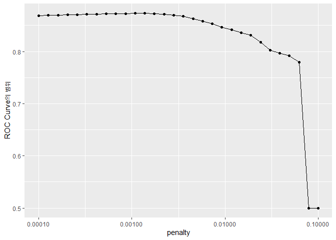
penalty가 적을수록 모델이 더 잘 작동한다는 것을 보여주네요.
그리고 오른쪽으로 갈수록 가파르게 ROC가 떨어지는 것을 볼 수 있습니다. 이것은 어느 정도 penalty가 높아지면, 모든 변수를 다 제거해버리기 때문입니다.
대체로 작은 penalty에서 좋은 효율을 보이므로 show_best를 통해 정리하겠습니다.

top_models <- 
  lr_res %>% 
  show_best('roc_auc', n = 15) %>% 
  arrange(penalty)

select_best함수를 사용해서 가장 좋은 모델을 고를 수도 있습니다. 하지만 같은 ROC_AUC 라면 penalty가 높을수록 좋습니다. 왜냐하면 관련없는 변수들이 penalty가 높을수록 잘 제거되기 때문입니다. 그래서 아래 그림과 같이, 비슷한 성능의 모델이라면 더 높은 패널티의 모델을 선택합니다.

lr_plot_lines

그럼 모델을 선정하고 시각화해보겠습니다.

lr_best <- 
  lr_res %>% 
  collect_metrics() %>% 
  arrange(penalty) %>% 
  slice(12)

lr_best

## # A tibble: 1 x 7
##   penalty .metric .estimator  mean     n std_err .config              
##     <dbl> <chr>   <chr>      <dbl> <int>   <dbl> <chr>                
## 1 0.00137 roc_auc binary     0.873     1      NA Preprocessor1_Model12

penalty가 12인 모델을 골라냅니다.

lr_auc <- 
  lr_res %>% 
  collect_predictions(parameters = lr_best) %>% 
  roc_curve(children, .pred_children) %>% 
  mutate(model = "Logistic Regression")

autoplot(lr_auc)

autoplot1

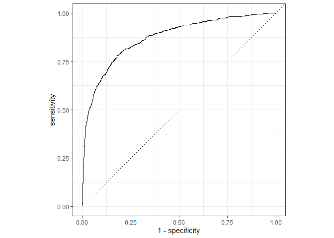
준수한 결과를 나타냅니다. 다음은 tree-based ensemble 모델을 사용해보겠습니다.

Tree Based Ensemble

Random foreset는 비교적 유연하고 효율적인 모델입니다. 그리고 종속변수에 상관없이 적용가능 하고, 적은 전처리 과정이 소요되므로 많은 분석가들이 선호합니다. 그럼 Random Forest를 사용해서 모델링을 수행해보겠습니다.

모델 구축과 Training 시간 단축

Random Forest는 Default 값의 Hyperparameter로도 준수한 결과를 냅니다. 이번에는 더 좋은 모델링을 위해서 튜닝을 수행하겠습니다. 이 과정의 단점은, Randon Forest에 사용되는 Tuning이 컴퓨팅 시간을 많이 소요한다는 점입니다. 이 단점을 보완하기 위해서 패키지에서 준비된 일정 함수를 사용하면, 모델 내에서 Computation을 core에 적절히 분할하여 할당할 수 있고, 이 결과로 Training 시간을 단축할 수 있습니다.

다만 이번에는 하나의 Validation Set만 있으므로, 굳이 병렬화하여 계산할 필요까지는 없습니다. 하지만 언젠가 병렬화해서 계산하려면 자신의 컴퓨터의 Core 수를 알고 있어야겠죠? 다행히도 R의 parallel 패키지에는 이를 도와주는 함수 detectCores()가 있습니다.

cores <- parallel::detectCores()
cores

## [1] 4

현재 제 컴퓨터에서는 4개의 코어를 가지고 있군요. 그래서 이런 코어 정보를 R의 모델에게 넘겨줄 수 있습니다.

rf_mod <- 
  rand_forest(mtry = tune(), min_n = tune(), trees = 1000) %>% 
  set_engine('ranger', num.threads = cores) %>% 
  set_mode('classification')

num.threads = cores를 통해서 앞서 정의한 컴퓨터의 core 수를 설정해줍니다.
그리고 mtry와 min_n을 hyperparameter 튜닝 대상으로 두겠습니다.

Recipe와 Workflow 만들기

Random Forest는 dummy가 필요없습니다.(너무 편하네요..) 대신 arrival_date를 가지고 Feature Engineering은 수행할 예정이므로 step을 통해 전처리를 해줍니다.

rf_recipe <- 
  recipe(children ~ ., data = hotel_other) %>% 
  step_date(arrival_date) %>% 
  step_holiday(arrival_date) %>% 
  step_rm(arrival_date) 

그리고 만든 Recipe를 Workflow에 태워줍니다.

rf_workflow <- 
  workflow() %>% 
  add_model(rf_mod) %>% 
  add_recipe(rf_recipe)

모델 훈련과 튜닝

rf_mod

## Random Forest Model Specification (classification)
## 
## Main Arguments:
##   mtry = tune()
##   trees = 1000
##   min_n = tune()
## 
## Engine-Specific Arguments:
##   num.threads = cores
## 
## Computational engine: ranger

rf_mod %>% 
  parameters()

## Collection of 2 parameters for tuning
## 
##  identifier  type    object
##        mtry  mtry nparam[?]
##       min_n min_n nparam[+]
## 
## Model parameters needing finalization:
##    # Randomly Selected Predictors ('mtry')
## 
## See `?dials::finalize` or `?dials::update.parameters` for more information.

mtry는 decistion tree가 보고 학습할 수 있는 변수의 개수를 1개 ~ 총 변수의 개수 사이만큼 정할 수 있습니다.
min_n은 node에서 갈라지는 최소한의 개수를 정합니다.

tune_grid를 사용해서 25개의 후보를 내보겠습니다.

set.seed(345)

rf_res <- 
  rf_workflow %>% 
  tune_grid(val_set,
            grid = 25,
            control = control_grid(save_pred = T),
            metrics = metric_set(roc_auc))

## i Creating pre-processing data to finalize unknown parameter: mtry

상위 5개의 모델만 추려보겠습니다.

rf_res %>% 
  show_best(metric = 'roc_auc')

## # A tibble: 5 x 8
##    mtry min_n .metric .estimator  mean     n std_err .config              
##   <int> <int> <chr>   <chr>      <dbl> <int>   <dbl> <chr>                
## 1     4     5 roc_auc binary     0.926     1      NA Preprocessor1_Model22
## 2     6    11 roc_auc binary     0.924     1      NA Preprocessor1_Model09
## 3     6    15 roc_auc binary     0.923     1      NA Preprocessor1_Model07
## 4     8    10 roc_auc binary     0.923     1      NA Preprocessor1_Model24
## 5     4    24 roc_auc binary     0.923     1      NA Preprocessor1_Model06

Random Forest의 튜닝 결과가 로직스틱 회귀의 성능인 0.881 보다 훨씬 좋은 성능을 보여줍니다.

결과를 시각화하겠습니다.

autoplot(rf_res)

mtry와 min_n이 작을수록 좋은 성능을 보여주는 경향이 있네요.

그럼 ROC AUC의 성능에 맞게 가장 좋은 모델을 선정하겠습니다.

rf_best <- 
  rf_res %>% 
  select_best(metric = 'roc_auc')
rf_best

## # A tibble: 1 x 3
##    mtry min_n .config              
##   <int> <int> <chr>                
## 1     4     5 Preprocessor1_Model22

필요한 데이터로 ROC Curve를 사용하기 위해 collect_prediction()을 수행하겠습니다. 이 함수는 control_grid(save_pred =TRUE)일 때만 사용 가능합니다.

rf_res %>% 
  collect_predictions()

## # A tibble: 187,475 x 8
##    id         .pred_children .pred_none  .row  mtry min_n children .config              
##    <chr>               <dbl>      <dbl> <int> <int> <int> <fct>    <chr>                
##  1 validation       0             1         1     9    14 none     Preprocessor1_Model01
##  2 validation       0             1        16     9    14 none     Preprocessor1_Model01
##  3 validation       0.000450      1.00     21     9    14 none     Preprocessor1_Model01
##  4 validation       0             1        31     9    14 none     Preprocessor1_Model01
##  5 validation       0.00675       0.993    33     9    14 none     Preprocessor1_Model01
##  6 validation       0.0535        0.947    45     9    14 none     Preprocessor1_Model01
##  7 validation       0.0273        0.973    46     9    14 none     Preprocessor1_Model01
##  8 validation       0.0393        0.961    53     9    14 none     Preprocessor1_Model01
##  9 validation       0.0816        0.918    58     9    14 none     Preprocessor1_Model01
## 10 validation       0.00278       0.997    60     9    14 none     Preprocessor1_Model01
## # ... with 187,465 more rows

앞에 두 개의 .pred으로 시작하는 컬럼이 있습니다. 두 컬럼이 각각 어떤 확률을 가지고 있었는지를 나타내줍니다. 그리고 이 컬럼 중 높은 값이 종속변수의 결과값으로 선정됩니다.

best random forest 모델을 사용하기 위해 parameter를 사용합니다.

rf_auc <- 
  rf_res %>% 
  collect_predictions(parameters = rf_best) %>% 
  roc_curve(children, .pred_children) %>% 
  mutate(model = 'Random Forest')

이제 로지스틱 회귀와 Random Forest의 ROC Curve를 비교해봅시다.

bind_rows(rf_auc, lr_auc) %>% 
  ggplot(aes(x = 1 - specificity, y = sensitivity, col = model))+
  geom_path(lwd = 1.5, alpha = 0.6)+
  geom_abline(lty = 3) +
  coord_equal()

roc_curv_compare

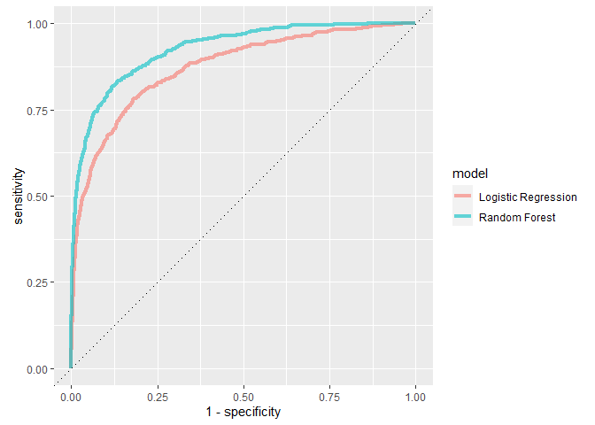
Random Forest가 항상 더 나은 성능을 보이는 것을 알 수 있군요

The Last Fit

분석의 목표는 어떤 호텔에 자녀와 같이 온 가족이 머무는지에 대한 예측이었습니다. Random Forest 모델이 모든 면에서 나은 성적을 보이므로, Random Forest 모델을 사용하겠습니다. 가장 좋은 Hyperparameter를 사용한 모델로 Training Data(train + validation)을 사용하여 Testing Data를 예측합니다.

parsnip 모델부터 적용하겠습니다. 여기서 importance = 'impurity'라는 새로운 인자를 추가할 예정입니다. 이 인자는 Variance Importance를 제공해주며 어떤 변수가 모델에 영향을 주는지 확인할 수 있게 해줍니다.

# Model
last_rf_mod <- 
  rand_forest(mtry = 8, min_n = 7, trees =1000) %>% 
  set_engine('ranger', num.threads = cores, importance = 'impurity') %>% 
  set_mode('classification')

# Workflow
last_rf_workflow <- 
  rf_workflow %>% 
  # 위에서 만든 모델을 새로 업데이트
  update_model(last_rf_mod)

# Last Fit
set.seed(345)
last_rf_fit <- 
  last_rf_workflow %>% 
  last_fit(splits)

last_rf_fit

## # Resampling results
## # Manual resampling 
## # A tibble: 1 x 6
##   splits                id               .metrics         .notes           .predictions          .workflow
##   <list>                <chr>            <list>           <list>           <list>                <list>   
## 1 <split [37500/12500]> train/test split <tibble [2 x 4]> <tibble [0 x 1]> <tibble [12,500 x 6]> <workflo~

위에서 작성한 workflow에는 모든 게 들어있습니다. Validation Set에서 나왔던 ROC AUC와 비슷한 값이 나올까요? 정리된 데이터를 뽑아내보겠습니다.

last_rf_fit %>% 
  collect_metrics()

## # A tibble: 2 x 4
##   .metric  .estimator .estimate .config             
##   <chr>    <chr>          <dbl> <chr>               
## 1 accuracy binary         0.945 Preprocessor1_Model1
## 2 roc_auc  binary         0.925 Preprocessor1_Model1

Validation set에서 봤던 ROC AUC와 비슷한 숫자가 나왔습니다.
이는 Validation Set으로 훈련시킨 모델이 새로운 데이터에도 잘 작동한다는 것을 의미합니다.

이제 Variance Importance를 살펴보겠습니다.

last_rf_fit %>% 
  pluck(".workflow",1 ) %>% 
  pull_workflow_fit() %>% 
  vip(num_features = 20)

workflow1

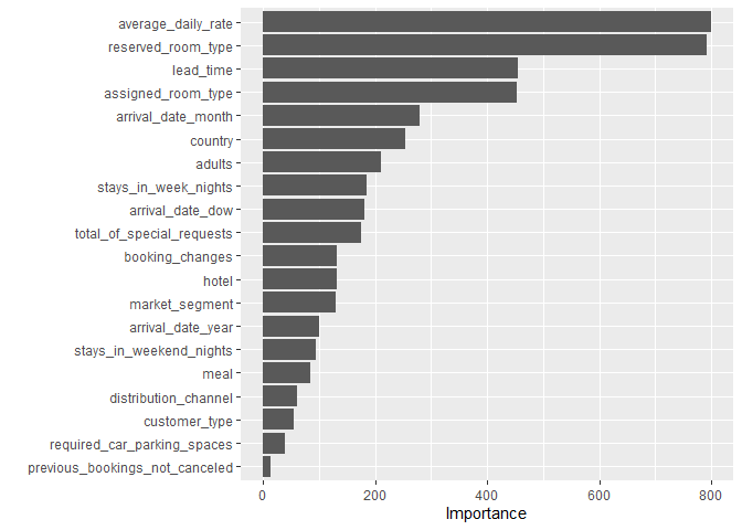
last_rf_fit에서 .workflow 컬럼을 통해 Variance Importance 정보를 얻을 수 있습니다.
pluck은 purrr패키지의 인덱싱 함수입니다.
가장 중요한 변수는 당일의 방 가격, 예약한 룸의 타입, 배정된 룸의 타입 등이군요.

Test Set을 바탕으로 ROC Curve를 그려봅시다. (이전 ROC Curve는 Validatoin Set으로 측정했습니다.)

last_rf_fit %>% 
  collect_predictions() %>% 
  roc_curve(children, .pred_children) %>% 
  autoplot()

autoplot2

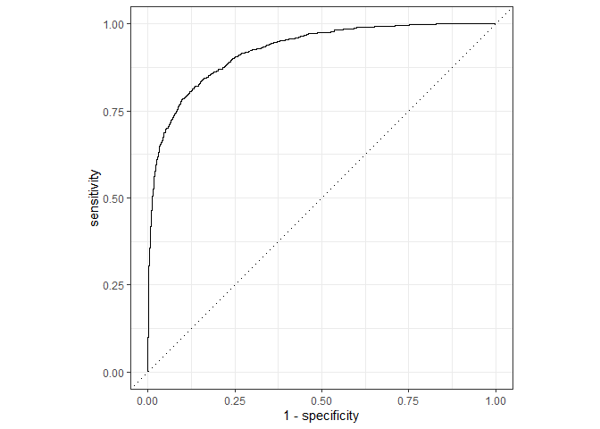
결과가 Validation set과 비슷합니다. 우리가 선택한 Hyper Parameter로 새로운 데이터에서도 준수하게 모델링이 작동됨을 알 수 있습니다.

마무리

1. Tidymodels를 정리하면서 느낀점

아직 정착이 완전하게 되지는 않은 신생 패키지이지만 잘 만든 것 같다는 생각이 듭니다. 무엇보다 R에서 하나의 포멧으로 여러 머신러닝 모델을 접근할 수 있다는 사실이 가장 마음에 드는 것 같습니다.
하지만 따라가야 할 함수와 프로세스가 아직 익숙하지 않군요. 처음 시작하는 분들에게는 약간의 허들이 될 수 있겠네요.

2. 앞으로의 계획

Tidymodels를 꾸준히 활용해서 Kaggle의 문제들을 해결해나갈 예정입니다. 해결해나가는 과정과 시행착오를 이 블로그에 꾸준히 여러분들과 공유하고 싶습니다.
Python이 확실히 머신러닝과 딥러닝에서는 대세를 잡은 것 같습니다. 아직은 시기상조이지만, 언젠가는 저도 파이썬을 배워서 다른 분석가, 또는 개발자들과 소통해야 하는 때가 오겠지요. 하지만 완벽히 R로 머신러닝의 프로세스를 익히고 파이썬을 보조로 사용하고 싶은 생각입니다.
쏘프라이즈라는 플랫폼을 접했습니다. 흥미로운 질문을 던지고, 그것을 데이터로 설명해야 하는 재미있는 프로젝트인 것 같습니다. 저 문제들을 함께 풀어보면서 R과 더 친해지고, 또 그 과정 역시 여기에 정리해볼게요 :)

수고하셨습니다!

The End.