Tidymodels로 시작하는 머신러닝 (4)
in DATA on Data, Machine Learning, Tidymodels, Fold, Tidymodels-recipe, 타이디모델, R-machine-learning, R, Cross-validation, 교차검증
개요
- Tuning을 통해 hyperparameter를 학습하는 방법을 익힙니다.
- Tidymodels - Tune Model Parameters 공식 영문서를 참고하여 만들었습니다.
- 관련 포스트
- 목차
튜닝이 필요한 이유
모델의 parameter 중에는 학습되지 않는 것들이 있습니다. 이런 parameter를 hyperparameter라고 부릅니다. 예를 들어서 random forest 모델에서의 mtry(의사결정 나무의 개수)는 분석가가 정합니다. 이것은 데이터를 통해 학습되는 영역이 아닙니다.
하지만, Performance 측면에서 가장 좋은 성능을 측정함으로써 최선의 hyperparameter를 정할 수 있습니다. 이 과정을 tuning이라고 하죠. 그럼 Step by Step으로 따라가 보겠습니다.
Library Call
library(tidymodels)

# Helper packages
library(modeldata)   # data Import
library(vip)         # Variance Importance 측정
library(tidyverse)
Data Load
data(cells, package = "modeldata")
cells
## # A tibble: 2,019 x 58
##    case  class angle_ch_1 area_ch_1 avg_inten_ch_1 avg_inten_ch_2 avg_inten_ch_3
##    <fct> <fct>      <dbl>     <int>          <dbl>          <dbl>          <dbl>
##  1 Test  PS        143.         185           15.7           4.95           9.55
##  2 Train PS        134.         819           31.9         207.            69.9
##  3 Train WS        107.         431           28.0         116.            63.9
##  4 Train PS         69.2        298           19.5         102.            28.2
##  5 Test  PS          2.89       285           24.3         112.            20.5
##  6 Test  WS         40.7        172          326.          654.           129.
##  7 Test  WS        174.         177          260.          596.           124.
##  8 Test  PS        180.         251           18.3           5.73          17.2
##  9 Test  WS         18.9        495           16.1          89.5           13.7
## 10 Test  WS        153.         384           17.7          89.9           20.4
## # ... with 2,009 more rows, and 51 more variables: avg_inten_ch_4 <dbl>,
## #   convex_hull_area_ratio_ch_1 <dbl>, convex_hull_perim_ratio_ch_1 <dbl>,
## #   diff_inten_density_ch_1 <dbl>, diff_inten_density_ch_3 <dbl>,
## #   diff_inten_density_ch_4 <dbl>, entropy_inten_ch_1 <dbl>, entropy_inten_ch_3 <dbl>,
## #   entropy_inten_ch_4 <dbl>, eq_circ_diam_ch_1 <dbl>, eq_ellipse_lwr_ch_1 <dbl>,
## #   eq_ellipse_oblate_vol_ch_1 <dbl>, eq_ellipse_prolate_vol_ch_1 <dbl>,
## #   eq_sphere_area_ch_1 <dbl>, eq_sphere_vol_ch_1 <dbl>, fiber_align_2_ch_3 <dbl>,
## #   fiber_align_2_ch_4 <dbl>, fiber_length_ch_1 <dbl>, fiber_width_ch_1 <dbl>,
## #   inten_cooc_asm_ch_3 <dbl>, inten_cooc_asm_ch_4 <dbl>,
## #   inten_cooc_contrast_ch_3 <dbl>, inten_cooc_contrast_ch_4 <dbl>,
## #   inten_cooc_entropy_ch_3 <dbl>, inten_cooc_entropy_ch_4 <dbl>,
## #   inten_cooc_max_ch_3 <dbl>, inten_cooc_max_ch_4 <dbl>, kurt_inten_ch_1 <dbl>,
## #   kurt_inten_ch_3 <dbl>, kurt_inten_ch_4 <dbl>, length_ch_1 <dbl>,
## #   neighbor_avg_dist_ch_1 <dbl>, neighbor_min_dist_ch_1 <dbl>,
## #   neighbor_var_dist_ch_1 <dbl>, perim_ch_1 <dbl>, shape_bfr_ch_1 <dbl>,
## #   shape_lwr_ch_1 <dbl>, shape_p_2_a_ch_1 <dbl>, skew_inten_ch_1 <dbl>,
## #   skew_inten_ch_3 <dbl>, skew_inten_ch_4 <dbl>, spot_fiber_count_ch_3 <int>,
## #   spot_fiber_count_ch_4 <dbl>, total_inten_ch_1 <int>, total_inten_ch_2 <dbl>,
## #   total_inten_ch_3 <int>, total_inten_ch_4 <int>, var_inten_ch_1 <dbl>,
## #   var_inten_ch_3 <dbl>, var_inten_ch_4 <dbl>, width_ch_1 <dbl>
Cell Image Data 이미지 분류
Decision tree 모델이 가지는 hyperparameter가 있습니다.
- Parameter 복잡도(
cost_complexity) - 최대 트리 깊이 (
tree_depth)
Decision tree 모델은 과적합(overfit)하는 경향이 있습니다. 왜냐하면 하나의 Decision Tree는 데이터가 100%로 잘 분류될 때 까지 최적의 트리를 나누기 때문입니다. 너무 훈련을 잘해서 Training Set으로 모델을 적합하면 안좋은 결과가 나오기도 합니다.
이런 과적합을 피하기 위해 pruning을 통해 cost_complexity를 튜닝하겠습니다. pruning은 한국어로 ’가지치기’정도로 해석될 수 있습니다. Decision Tree에서 불필요하게 늘어나는 가지를 쳐내는 것으로 이해하면 좋을 것 같네요. pruning은 모델이 복잡해질수록 패널티를 부여합니다. cost_complexity가 0에 가까울수록 pruning되는 노드들이 저어지면서, 과적합의 비율이 높아집니다.
그런데 반대로 pruning 과정이 지나치면, 다른 문제가 발생합니다. 바로 과소적합(underfit)입니다. 이 현상을 막아주는 역할을 하는 hyperparameter가 바로 tree_depth입니다. 일정한 tree가 생성되었다면 적정 지점에서 멈춰야겠죠? 이렇게 cost_complexity와 tree_depth의 hyperparameter tuning을 진행해서 최적의 이미지 분류를 진행해보겠습니다.
Data Split
set.seed(123)
cell_split <- initial_split(cells %>% select(-case), strata = class)

cell_train <- training(cell_split)
cell_train <- testing(cell_split)
Tuning HyperParameters
parsnip패키지를 통해 Decision tree 모델링을 수행합니다. cost_complexity와 tree_depth는 tuning의 대상이므로 tune()으로 지정해놓습니다. 표시만 이렇게 해놓는 것이며 나중에 tuning을 마치면 단일값을 입력할 예정입니다.
tune_spec <-
  decision_tree(
    cost_complexity = tune(),
    tree_depth = tune()
  ) %>%
  set_engine("rpart") %>%
  set_mode("classification")
앞서 설명했듯, Dataset으로 어떤 값이 hyperparameter로 사용되어야하는지 알 수는 없습니다. 단, resample을 통해 어떤 모델이 더 나은 결과가 나오는지를 판단할 수는 있습니다.
tree_grid <- grid_regular(cost_complexity(),
                          tree_depth(),
                          levels = 5)

tree_grid
## # A tibble: 25 x 2
##    cost_complexity tree_depth
##              <dbl>      <int>
##  1    0.0000000001          1
##  2    0.0000000178          1
##  3    0.00000316            1
##  4    0.000562              1
##  5    0.1                   1
##  6    0.0000000001          4
##  7    0.0000000178          4
##  8    0.00000316            4
##  9    0.000562              4
## 10    0.1                   4
## # ... with 15 more rows
grid_regular는 dial패키지의 함수입니다.- parameter objetct를 위해 Random한 Grid를 생성해주는 함수입니다.
- levels = 5는 5개씩 grid를 출력해달라는 뜻입니다.
- 두 개의 파라미터에 대한 요청을 했으므로, 5*5 = 25개의 Grid를 출력합니다.
tree_grid %>%
  count(tree_depth)
## # A tibble: 5 x 2
##   tree_depth     n
## *      <int> <int>
## 1          1     5
## 2          4     5
## 3          8     5
## 4         11     5
## 5         15     5
이제 25 개의 Tree Model 후보가 있으니, 각각 교차검증을 수행해보겠습니다.
set.seed(234)
cell_folds <- vfold_cv(cell_train)
tuning은 rsample 패키지를 사용합니다.
Grid를 통한 모델 튜닝
tune_grid함수는 그리드 서치를 수행하는 함수입니다. 해당 함수를 사용해서 튜닝을 수행하겠습니다.
- GridSearch를 잘 설명한 포스트
- 이전 포스트에서 사용했던
workflow를 활용하겠습니다. 링크
set.seed(345)

tree_wf <- workflow() %>%
  add_model(tune_spec) %>%
  add_formula(class ~ .)

tree_res <-
  tree_wf %>%
  tune_grid(
    resamples = cell_folds,
    grid = tree_grid
  )

tree_res
## # Tuning results
## # 10-fold cross-validation
## # A tibble: 10 x 4
##    splits           id     .metrics          .notes
##    <list>           <chr>  <list>            <list>
##  1 <split [453/51]> Fold01 <tibble [50 x 6]> <tibble [0 x 1]>
##  2 <split [453/51]> Fold02 <tibble [50 x 6]> <tibble [0 x 1]>
##  3 <split [453/51]> Fold03 <tibble [50 x 6]> <tibble [0 x 1]>
##  4 <split [453/51]> Fold04 <tibble [50 x 6]> <tibble [0 x 1]>
##  5 <split [454/50]> Fold05 <tibble [50 x 6]> <tibble [0 x 1]>
##  6 <split [454/50]> Fold06 <tibble [50 x 6]> <tibble [0 x 1]>
##  7 <split [454/50]> Fold07 <tibble [50 x 6]> <tibble [0 x 1]>
##  8 <split [454/50]> Fold08 <tibble [50 x 6]> <tibble [0 x 1]>
##  9 <split [454/50]> Fold09 <tibble [50 x 6]> <tibble [0 x 1]>
## 10 <split [454/50]> Fold10 <tibble [50 x 6]> <tibble [0 x 1]>
tune_grid는 시간이 오래 걸립니다.. :)- 튜닝이 완료되면
collect_metrics를 통해 깔끔하게 결과를 볼 수 있습니다.
tree_res %>%
  collect_metrics()
## # A tibble: 50 x 8
##    cost_complexity tree_depth .metric  .estimator  mean     n std_err .config
##              <dbl>      <int> <chr>    <chr>      <dbl> <int>   <dbl> <chr>
##  1    0.0000000001          1 accuracy binary     0.754    10  0.0161 Preprocessor1_Mode~
##  2    0.0000000001          1 roc_auc  binary     0.741    10  0.0129 Preprocessor1_Mode~
##  3    0.0000000178          1 accuracy binary     0.754    10  0.0161 Preprocessor1_Mode~
##  4    0.0000000178          1 roc_auc  binary     0.741    10  0.0129 Preprocessor1_Mode~
##  5    0.00000316            1 accuracy binary     0.754    10  0.0161 Preprocessor1_Mode~
##  6    0.00000316            1 roc_auc  binary     0.741    10  0.0129 Preprocessor1_Mode~
##  7    0.000562              1 accuracy binary     0.754    10  0.0161 Preprocessor1_Mode~
##  8    0.000562              1 roc_auc  binary     0.741    10  0.0129 Preprocessor1_Mode~
##  9    0.1                   1 accuracy binary     0.754    10  0.0161 Preprocessor1_Mode~
## 10    0.1                   1 roc_auc  binary     0.741    10  0.0129 Preprocessor1_Mode~
## # ... with 40 more rows
아래와 같이 그래프를 그려봅시다.
tree_res %>%
  collect_metrics() %>%
  # tree depth를 factor로 치환
  mutate(tree_depth = factor(tree_depth)) %>%
  ggplot(aes(cost_complexity, mean, color = tree_depth))+
  geom_line(alpha = 0.6)+
  geom_point(size = 2)+
  # metric을 차원으로 그래프를 두 개로 나눔
  facet_wrap( ~ .metric, scales = 'free', nrow = 2)+
  # log scale을 적용
  scale_x_log10(labels = scales::label_number()) # Decimal Format으로 강제함
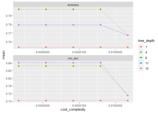
가장 아래에 있는 모델은 tree가 하나일 때입니다. 가장 안좋은 성능을 보이는 것 같네요. 반대로 tree가 8인 모델이 가장 좋은 성능을 보이는 것 같습니다. show_best()함수로 가장 좋은 모델을 추려낼 수 있습니다.
tree_res %>%
  show_best("roc_auc")
## # A tibble: 5 x 8
##   cost_complexity tree_depth .metric .estimator  mean     n std_err .config
##             <dbl>      <int> <chr>   <chr>      <dbl> <int>   <dbl> <chr>
## 1    0.0000000001          8 roc_auc binary     0.841    10  0.0169 Preprocessor1_Model11
## 2    0.0000000178          8 roc_auc binary     0.841    10  0.0169 Preprocessor1_Model12
## 3    0.00000316            8 roc_auc binary     0.841    10  0.0169 Preprocessor1_Model13
## 4    0.000562              8 roc_auc binary     0.841    10  0.0169 Preprocessor1_Model14
## 5    0.0000000001         11 roc_auc binary     0.841    10  0.0169 Preprocessor1_Model16
best_tree <- tree_res %>%
  select_best("roc_auc")

best_tree
## # A tibble: 1 x 3
##   cost_complexity tree_depth .config
##             <dbl>      <int> <chr>
## 1    0.0000000001          8 Preprocessor1_Model11
여기서 도출된 cost_complexity와 tree_depth가 AUC를 최대값으로 가지는군요. 제일 좋은 성능을 보이는 Hyperparameter인 것 같습니다.
Finalizing Model
이제 최종적으로 튜닝된 Hyperparameter를 모델에 적용해봅시다.
final_wf <-
  tree_wf %>%
  finalize_workflow(best_tree)

final_wf
## == Workflow =============================================================================
## Preprocessor: Formula
## Model: decision_tree()
##
## -- Preprocessor -------------------------------------------------------------------------
## class ~ .
##
## -- Model --------------------------------------------------------------------------------
## Decision Tree Model Specification (classification)
##
## Main Arguments:
##   cost_complexity = 1e-10
##   tree_depth = 8
##
## Computational engine: rpart
워크플로우에 정상적으로 적용된 것으로 보입니다. 이제 훈련 데이터를 우리의 모델에 학습시켜봅시다.
final_tree <-
  final_wf %>%
  fit(data = cell_train)

final_wf
## == Workflow =============================================================================
## Preprocessor: Formula
## Model: decision_tree()
##
## -- Preprocessor -------------------------------------------------------------------------
## class ~ .
##
## -- Model --------------------------------------------------------------------------------
## Decision Tree Model Specification (classification)
##
## Main Arguments:
##   cost_complexity = 1e-10
##   tree_depth = 8
##
## Computational engine: rpart
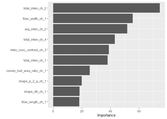
이 결과에서 우리는 Variance Importance를 볼 수 있습니다. 즉 이 모델에서 종요도가 높은 변수가 어떤 변수였는지 살펴볼 수 있는 방법인데요, vip패키지를 사용합니다.
library(vip)

final_tree %>%
  pull_workflow_fit() %>%
  vip()
The Last Fit
이제 최종결과를 Fitting 해보겠습니다.
final_fit <-
  final_wf %>%
  # recipe로 나누었던 cell_split에 대하여 Last_fit함수 적용
  last_fit(cell_split)

final_fit %>%
  collect_metrics()
## # A tibble: 2 x 4
##   .metric  .estimator .estimate .config
##   <chr>    <chr>          <dbl> <chr>
## 1 accuracy binary         0.794 Preprocessor1_Model1
## 2 roc_auc  binary         0.851 Preprocessor1_Model1
final_fit %>%
  # 예측결과 도출
  collect_predictions() %>%
  # ROC Cure 도출
  roc_curve(class, .pred_PS) %>%
  # Plot 그리기
  autoplot()
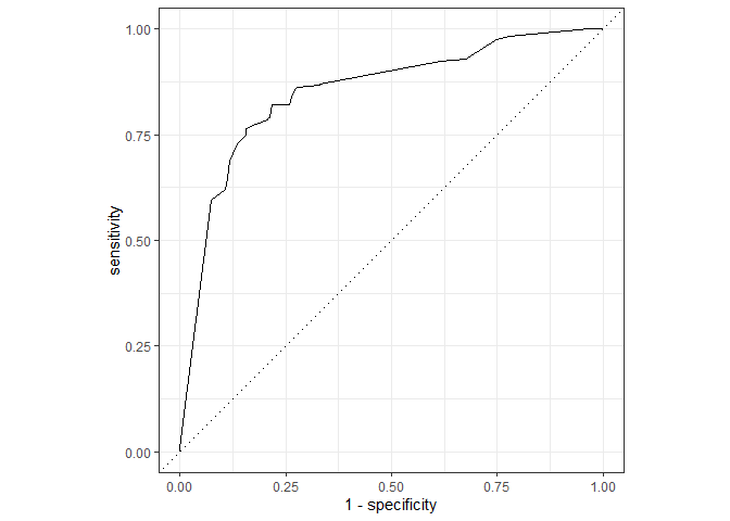
ROC 결과를 보니 과적합된 결과는 없어보이네요. 이로써 Tuning 과정을 마치겠습니다.
last_fit함수는 final model을 훈련데이터에 fitting 하고 테스트 데이터에 적용하는 함수입니다.- 아레에는 더 많은 hyperparameter에 대한 정보와 모델 정보를 링크해두었습니다. 참고하세요!