Tidymodels로 시작하는 머신러닝 (2)
in DATA on Data, Machine Learning, Tidymodels, Recipe, Tidymodels-recipe, 타이디모델-레시피, R-machine-learning, R
개요
- Recipe의 전반적인 개념에 대해서 설명합니다.
- 본 문서는 tidymodels 공식 영문서를 참고로 만들었습니다.
- 이전포스트 - Tidymodel로 모델 만들기
- 관련 포스트
- 목차
Recipe
Recipe는 머신러닝 프로세스에서 데이터의 전처리를 도와주는 tidymodel의 전처리 패키지입니다. 아래와 같은 기능을 포함합니다.
- Qualitative Variable(질적 변수)의 dummy Variable(더미변수) 로의 변환(질적 변수는 Categorical Variable로 부르기도 합니다.)
- Feature Scaling
- 서로 다른 단위를 가지고 있는 데이터를 정규화해주는 과정
- 한 번에 모든 Variable을 변경
- Key Feature만 뽑아내기
- 참고자료
library(tidymodels)      # 기본 패키지

# Helper packages
library(nycflights13)    # flight data를 위해 로드
library(skimr)           # 데이터 구조 살필 때 필요한 패키지
Flight Data
flights 데이터는 뉴욕의 비행 출발/도착과 관련된 데이터입니다. 이 데이터를 통해서 어떤 비행기가 30분 연착할 지를 예측해보는 과정을 수행해보겠습니다.
먼저 데이터를 살펴봐야겠군요. 앞으로는 두 개의 테이블을 사용할 예정입니다.
flights
## # A tibble: 336,776 x 19
##     year month   day dep_time sched_dep_time dep_delay arr_time sched_arr_time arr_delay carrier flight tailnum
##    <int> <int> <int>    <int>          <int>     <dbl>    <int>          <int>     <dbl> <chr>    <int> <chr>
##  1  2013     1     1      517            515         2      830            819        11 UA        1545 N14228
##  2  2013     1     1      533            529         4      850            830        20 UA        1714 N24211
##  3  2013     1     1      542            540         2      923            850        33 AA        1141 N619AA
##  4  2013     1     1      544            545        -1     1004           1022       -18 B6         725 N804JB
##  5  2013     1     1      554            600        -6      812            837       -25 DL         461 N668DN
##  6  2013     1     1      554            558        -4      740            728        12 UA        1696 N39463
##  7  2013     1     1      555            600        -5      913            854        19 B6         507 N516JB
##  8  2013     1     1      557            600        -3      709            723       -14 EV        5708 N829AS
##  9  2013     1     1      557            600        -3      838            846        -8 B6          79 N593JB
## 10  2013     1     1      558            600        -2      753            745         8 AA         301 N3ALAA
## # ... with 336,766 more rows, and 7 more variables: origin <chr>, dest <chr>, air_time <dbl>, distance <dbl>,
## #   hour <dbl>, minute <dbl>, time_hour <dttm>
weather
## # A tibble: 26,115 x 15
##    origin  year month   day  hour  temp  dewp humid wind_dir wind_speed wind_gust precip pressure visib
##    <chr>  <int> <int> <int> <int> <dbl> <dbl> <dbl>    <dbl>      <dbl>     <dbl>  <dbl>    <dbl> <dbl>
##  1 EWR     2013     1     1     1  39.0  26.1  59.4      270      10.4         NA      0    1012     10
##  2 EWR     2013     1     1     2  39.0  27.0  61.6      250       8.06        NA      0    1012.    10
##  3 EWR     2013     1     1     3  39.0  28.0  64.4      240      11.5         NA      0    1012.    10
##  4 EWR     2013     1     1     4  39.9  28.0  62.2      250      12.7         NA      0    1012.    10
##  5 EWR     2013     1     1     5  39.0  28.0  64.4      260      12.7         NA      0    1012.    10
##  6 EWR     2013     1     1     6  37.9  28.0  67.2      240      11.5         NA      0    1012.    10
##  7 EWR     2013     1     1     7  39.0  28.0  64.4      240      15.0         NA      0    1012.    10
##  8 EWR     2013     1     1     8  39.9  28.0  62.2      250      10.4         NA      0    1012.    10
##  9 EWR     2013     1     1     9  39.9  28.0  62.2      260      15.0         NA      0    1013.    10
## 10 EWR     2013     1     1    10  41    28.0  59.6      260      13.8         NA      0    1012.    10
## # ... with 26,105 more rows, and 1 more variable: time_hour <dttm>
- weather 데이터는 날씨 데이터입니다. flights 데이터와는
origin과time_hour컬럼을 공유합니다.
데이터를 로드해보겠습니다.
set.seed(123)

flight_data <-
  flights %>%
  # arr_delay라는 범주형 종속변수 만들기
  mutate(arr_delay = ifelse(arr_delay < 30,'on_time','late'),
         arr_delay = factor(arr_delay),
         # YYYY-MM-DD 데이터로 치환
         date = as.Date(time_hour)
       ) %>%
  # Weather Data와 Origin(출발지), time_hour(일자,시간) 을 키로 inner join 수행행
  inner_join(weather, by = c('origin','time_hour')) %>%
  # 필요한 컬럼만 가져오기
  select(dep_time, flight, origin, dest, air_time, distance,
         carrier, date, arr_delay, time_hour) %>%
  # Missing Data가 있는 열은 삭제
  na.omit() %>%
  mutate_if(is.character, as.factor)
그리고 연착된 비행기가 몇 퍼센트인지 살펴봅시다.
flight_data %>%
  count(arr_delay) %>%
  mutate(prop = n/sum(n))
## # A tibble: 2 x 3
##   arr_delay      n  prop
## * <fct>      <int> <dbl>
## 1 late       52540 0.161
## 2 on_time   273279 0.839
- 우리는 비행기의 연착 여부를 종속변수로 하므로, Logistic Regression을 수행해야 함을 염두해둡시다.
skim이라는 함수를 통해서 데이터의 구조를 편하게 파악할 수 있습니다.
flight_data %>%
  skim(dest, carrier)
| Name | Piped data |
| Number of rows | 325819 |
| Number of columns | 10 |
| _______________________ | |
| Column type frequency: | |
| factor | 2 |
| ________________________ | |
| Group variables | None |
Data summary
Variable type: factor
| skim_variable | n_missing | complete_rate | ordered | n_unique | top_counts |
|---|---|---|---|---|---|
| dest | 0 | 1 | FALSE | 104 | ATL: 16771, ORD: 16507, LAX: 15942, BOS: 14948 |
| carrier | 0 | 1 | FALSE | 16 | UA: 57489, B6: 53715, EV: 50868, DL: 47465 |
- dest 변수에는 약 104개의 값이 있는 것을 확인할 수 있습니다.
- 우리가 원하는 것은 Logistic Regression입니다. 따라서 해당 머신러닝을 수행하기 위해서는, Nominal Variable이 Dummy Variable로 치환되어야 합니다.
- 이후 분석 과정에서 치환 과정을 차차 다루겠습니다.
Data Spliting
# Random 결과를 Fixing
set.seed(123)
# 3/4를 트레이닝 데이터로 사용
data_split <- initial_split(flight_data, prop = 3/4)

# 트레이닝 셋과 테스트 셋으로 데이터 나누기
train_data <- training(data_split)
test_data <- testing(data_split)
rsample이라는 패키지를 통해서 Data Split을 진행할 수 있습니다.
Recipe와 Role
flights_rec <-
  # formula와 data를 정의하여 recipe 구축
  recipe(formula = arr_delay ~ ., data = train_data) %>%
  # role update
  update_role(flight, time_hour, new_role = "ID")
formula를 통해서 식을 정의해줍니다. 여기서.은 모든predictor를 의미합니다.data를 통해서train_data를 지정합니다.
recipe안에서 role을 부여하거나 바꿀 때 사용합니다.flight와time_hour데이터는 여기서 ID라는 role을 부여받았습니다.(굳이 ID라는 문자열이 아니어도 됩니다.) 이렇게 함으로써 변수를 지우지 않고,flight와time_hour는formula에서 제외하도록recipe에게 알려주는 것입니다.
summary(flights_rec)
## # A tibble: 10 x 4
##    variable  type    role      source
##    <chr>     <chr>   <chr>     <chr>
##  1 dep_time  numeric predictor original
##  2 flight    numeric ID        original
##  3 origin    nominal predictor original
##  4 dest      nominal predictor original
##  5 air_time  numeric predictor original
##  6 distance  numeric predictor original
##  7 carrier   nominal predictor original
##  8 date      date    predictor original
##  9 time_hour date    ID        original
## 10 arr_delay nominal outcome   original
Feature Engineering
Feature Engineering은 머신러닝의 중요한 단계입니다. Feature Engineering이란 기존 데이터에서 유용한 컬럼을 뽑아내거나, 정제해내서 새로운 컬럼을 만들어 모델링을 향상시키는 활동을 의미합니다. 이 데이터에는 date 컬럼이 있습니다. 이는 날짜 데이터이며 type역시 날짜로 되어 있습니다.
flight_data %>%
  distinct(date) %>%
  mutate(numeric_date = as.numeric(date))
## # A tibble: 364 x 2
##    date       numeric_date
##    <date>            <dbl>
##  1 2013-01-01        15706
##  2 2013-01-02        15707
##  3 2013-01-03        15708
##  4 2013-01-04        15709
##  5 2013-01-05        15710
##  6 2013-01-06        15711
##  7 2013-01-07        15712
##  8 2013-01-08        15713
##  9 2013-01-09        15714
## 10 2013-01-10        15715
## # ... with 354 more rows
distinct를 통해서 유일한 데이터만 골라냅니다.as.numeric을 통해서 날짜 타입인 데이터를 숫자로 바꿔줍니다.- 이렇게 하는 이유는 날짜의 숫자형 데이터가 modeling과정에서 도움이 될 수 있기 때문입니다.(log odds비 등)
date자체를 사용하는 것도 좋지만,date에서 파생되는 년, 월, 주, 요일 등의 데이터로도 좋은 인사이트를 얻을 수 있습니다.- 위 과정이 Feature Engineering입니다. 원래 있는 데이터에서 새로운 데이터를 만들어내는 것!
flights_rec <-
  recipe(arr_delay ~ ., data = train_data) %>%
  update_role(flight, time_hour, new_role = "ID") %>%
  step_date(date, features = c("dow", "month")) %>%
  step_holiday(date, holidays = timeDate::listHolidays("US")) %>%
  step_rm(date)
step_date()는 Date Feature Genrator라고 불리우는recipe의 함수입니다.- 말 그대로 날짜를 생성하는 역할을 수행합니다.
dow는 day of week으로 요일을 의미하고,month는 당연히 월을 의미하겠죠?
step_holiday()함수는 휴일을 binary(또는 플래그) 형식으로 표현해주는 함수입니다.- 한국 공휴일을 사용하는 방법이 있을까요? 해당 내용은 나중에 찾으면 추가하겠습니다.
step_rm()을 통해 더이상 모델이 포함되길 원치 않는date컬럼을 삭제합니다.
이제 어떤 과정이 남았을까요? 저희는 Logistic Regression을 수행하길 원합니다. 그래서 모든 변수는 숫자 변수로 변경되어야 하고 Factor형태의 변수는 모두 dummy variable로 변경을 해줘야 합니다. 예를 들어서 orgin 변수 안에 EWR, JFK, LGA 세 개의 변수만 있다고 가정하면, 아래와 같이 dummy variable을 생성해줘야 합니다.
| ORIGIN | ORGIN_JFK | ORGIN_LGA |
|---|---|---|
| EWR | 0 | 0 |
| JFK | 1 | 0 |
| LGA | 0 | 1 |
recipe는 몇 가지 명령어로 dummy처리를 도와줍니다. 몇몇 패키지는 자동으로 dummy가 생성이 되도록 강제하는 경우도 있지만, recipe는 선택권을 줍니다. 이유는 아래와 같습니다.
- dummy variable이 필요하지 않을 수도 있는 경우
- dummy variable로 바꾸지 않았을 때 모델링 성능이 더 나은 경우
recipe는 step_dummy()함수를 통해 더미 변수를 생성합니다.
flights_rec <-
  recipe(arr_delay ~ ., data = train_data) %>%
  update_role(flight, time_hour, new_role = "ID") %>%
  step_date(date, features = c("dow", "month")) %>%
  step_holiday(date, holidays = timeDate::listHolidays("US")) %>%
  step_rm(date) %>%
  step_dummy(all_nominal(), -all_outcomes())
all_nominal()은 character 이거나 factor인 컬럼을 모두 골라냅니다.-all_outcomes()는recipestep에서 outcome variable을 모두 제외시킵니다.
이를 통해
step_dummy는 종속변수를 제외한 모든 character, factor 변수를 dummy화 합니다.
carrier와 dest의 경우 빈도가 적은 값이 있을 수 있습니다. 따라서 test_data의 값의 개수와 train_data에서 가지고 있는 유니크한 값의 개수가 다를 수 있죠. 이는 training_set에서는 없는 dummy_variable이 만들어질 가능성이 있다는 뜻입니다. 그래서 anti_join을 통해서 test_data에는 있지만, train_data에는 없는 값을 가져오겠습니다.
test_data %>%
  distinct(dest) %>%
  anti_join(train_data)
## Joining, by = "dest"

## # A tibble: 0 x 1
## # ... with 1 variable: dest <fct>
- Training_Set에
recipe를 적용하면 factor level이 flight_data(training_set이 아님)에서 나오기 때문에 LEX에 대한 컬럼이 만들어지지만, 이 열에는 모두 0이 나오게 됩니다.- <2021.05.13 추가> Set.seed 설정 실패로 __LEX__가 검출되지 않는 결과가 나왔습니다 :< 나왔다고 가정하고 생각해주세요!
- 이는 Zero Variance Predictor라고 불리며, 경우에 따라 경고 및 기타 문제를 유발하기도 합니다.
- 따라서
step_zv()를 통해 training_set에 단일 값이 있을 때 데이터에서 컬럼을 제거합니다. step_dummy()이후에 적용 시켜 줍니다.
flights_rec <-
  recipe(arr_delay ~ ., data = train_data) %>%
  update_role(flight, time_hour, new_role = "ID") %>%
  step_date(date, features = c("dow", "month")) %>%
  step_holiday(date, holidays = timeDate::listHolidays("US")) %>%
  step_rm(date) %>%
  step_dummy(all_nominal(), -all_outcomes()) %>%
  step_zv(all_predictors())
Recipe 모델적합
Logistic Fitting
지금까지 만든 Recipe를 바탕으로 Logistic Regression을 적합해보겠습니다.
lr_mod <-
  logistic_reg() %>%
  set_engine('glm')
이제 세 단계를 거쳐서 모델적합을 수행합니다.
Recipe로 Training_Set 처리하기- 어떤 변수가 dummy variable이 되는지를 결정합니다.
- 또한 어떤 변수가 zero-variance가 되어야 하는지를 결정합니다.
Recipe를 Training_Set에 적용하기Recipe를 Testing_Set에 적용하기
- 새로이 계산되거나 적용되는 것 없이 Training_Set에서의 dummy variable의 결과와 zero-variance의 결과가 Testing_Set에 적용됩니다.
Workflow 적용
Workflow는Recipe와 짝꿍입니다.Workflow를 통해서Recipe와model을 묶을 수 있습니다.굳이 이렇게 묶는 이유는 모델마다 다른
Recipe를 사용할 수 있기 때문입니다. 따라서Workflow라는 틀을 만들고 그 틀에Recipe와Model을 블럭처럼 끼워넣는다고 생각하시면 될 것 같습니다.
- 장점
- 각각의 Object를
workflow에 묶어놓으면 독립된 작업을 할 필요가 없이 간단해집니다. Recipe준비와 모델적합을fit()만으로 수행할 수 있습니다.- 뒤에서 나오게 될
tune이라는 parameter tuning과정과 연계됩니다. - 확률 수정이나 Classification Cut-Off와 같은 차후 프로세스를 지원합니다.
- 각각의 Object를
flights_wflow <-
  workflow() %>%
  add_model(lr_mod) %>%
  add_recipe(flights_rec)

flights_wflow
## == Workflow ===================================================================================================
## Preprocessor: Recipe
## Model: logistic_reg()
##
## -- Preprocessor -----------------------------------------------------------------------------------------------
## 5 Recipe Steps
##
## * step_date()
## * step_holiday()
## * step_rm()
## * step_dummy()
## * step_zv()
##
## -- Model ------------------------------------------------------------------------------------------------------
## Logistic Regression Model Specification (classification)
##
## Computational engine: glm
workflow에lr_mod와flights_rec을 차례로 붙여줍니다.
이제 앞서 장점에서 설명했듯, fit()함수 하나로 recipe와 model fitting을 수행합니다.
flights_fit <-
  flights_wflow %>%
  fit(data = train_data)
이제 최종 Reicpe와 Model은 flights_fit라는 객체 안에 있습니다. 이 객체에서 모델 또는 Recipe만 따로 뽑아내고 싶을 수 있습니다. 이 때 사용 하는 함수를 아래에 소개합니다.
pull_workflow_fit(): 모델만 추출pull_workflow_prepped_recipe():Recipe추출
flights_fit %>%
  pull_workflow_fit() %>%
  tidy()
## # A tibble: 158 x 5
##    term                         estimate std.error statistic  p.value
##    <chr>                           <dbl>     <dbl>     <dbl>    <dbl>
##  1 (Intercept)                   4.09    2.72           1.50 1.33e- 1
##  2 dep_time                     -0.00166 0.0000141   -118.   0.
##  3 air_time                     -0.0436  0.000563     -77.6  0.
##  4 distance                      0.00674 0.00150        4.50 6.83e- 6
##  5 date_USChristmasDay           1.08    0.171          6.29 3.27e-10
##  6 date_USColumbusDay            0.605   0.165          3.67 2.46e- 4
##  7 date_USCPulaskisBirthday      0.750   0.130          5.77 8.02e- 9
##  8 date_USDecorationMemorialDay  0.300   0.114          2.65 8.17e- 3
##  9 date_USElectionDay            0.581   0.166          3.50 4.57e- 4
## 10 date_USGoodFriday             1.21    0.159          7.60 2.92e-14
## # ... with 148 more rows
예측(Prediction)
지금까지의 과정은 모두 비행기 연착이 30분이 될 지 안 될지를 예측하기 위한 데이터 훈련과정이었습니다. 우리는
- 모델을 만들었습니다.(
lr_mod) - 전처리도 수행했습니다.(
flights_rec) - 모델과 전처리를 묶어서 프로세스를 만들었습니다.(
flights_wflow) - Traing_Data를 통해 Workflow를 훈련시켰습니다. (
fit())
이제는 우리가 predict()에 지금까지 만든 프로세스를 사용할 때가 되었습니다.
predict(flights_fit, test_data)
## # A tibble: 81,454 x 1
##    .pred_class
##    <fct>
##  1 on_time
##  2 on_time
##  3 on_time
##  4 on_time
##  5 on_time
##  6 on_time
##  7 on_time
##  8 on_time
##  9 on_time
## 10 on_time
## # ... with 81,444 more rows
- outcome variable이 Factor이므로
predict()의 결과도 late, on time 두 개의 값을 가진 Factor 변수를 출력합니다. - 만약 왜 late, on time이 나왔는지 확률값을 알고 싶다고 한다면,
type = "prob"을 통해 구현할 수 있습니다.
flights_pred <-
  predict(flights_fit, test_data, type = 'prob') %>%
  bind_cols(test_data %>% select(arr_delay, time_hour, flight))
flights_pred
## # A tibble: 81,454 x 5
##    .pred_late .pred_on_time arr_delay time_hour           flight
##         <dbl>         <dbl> <fct>     <dttm>               <int>
##  1    0.0590          0.941 on_time   2013-01-01 05:00:00   1714
##  2    0.00866         0.991 on_time   2013-01-01 05:00:00    725
##  3    0.0498          0.950 on_time   2013-01-01 06:00:00    301
##  4    0.0277          0.972 on_time   2013-01-01 06:00:00    194
##  5    0.0423          0.958 on_time   2013-01-01 06:00:00   1124
##  6    0.0961          0.904 late      2013-01-01 06:00:00   3768
##  7    0.0126          0.987 on_time   2013-01-01 06:00:00    709
##  8    0.0285          0.971 on_time   2013-01-01 06:00:00    575
##  9    0.0741          0.926 on_time   2013-01-01 06:00:00     27
## 10    0.0240          0.976 on_time   2013-01-01 06:00:00   4646
## # ... with 81,444 more rows
모델평가(Evaluation)
이제 모델 적합은 끝났습니다. 마지막으로 평가를 해야겠지요? 평가는 ROC Curve를 통해서 수행할 예정입니다. 그리고 yardstick 패키지의 함수를 사용할 예정입니다.
- Roc_Curve & Confusion Matrix : 정리가 한국어로 잘 되어있는 자료입니다. 혹시 해당 내용에 대해 공부하고 싶으신 분들은 참고하시면 좋을 것 같습니다 :)
ROC Curve
flights_pred %>%
  roc_curve(truth = arr_delay, .pred_late) %>%
  autoplot()
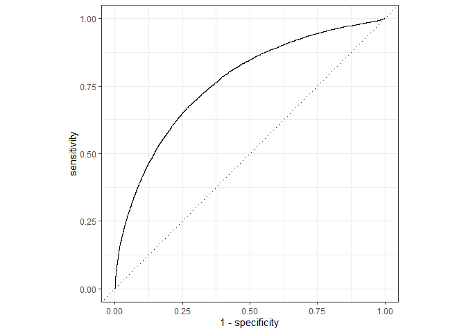
ROC_AUC
flights_pred %>%
  roc_auc(truth = arr_delay, .pred_late)
## # A tibble: 1 x 3
##   .metric .estimator .estimate
##   <chr>   <chr>          <dbl>
## 1 roc_auc binary         0.766
결과가 나쁘지 않습니다. 다음화에서는 Evaluation에 대해 더 깊이 다뤄보도록 하겠습니다.